Until this work, I had never performed any side channel attack on a device. Because I read a lot of papers and saw a lot of talks in conference about that, I thought I knew a lot about SCA.
However, when it comes to perform it for real, things get harder!
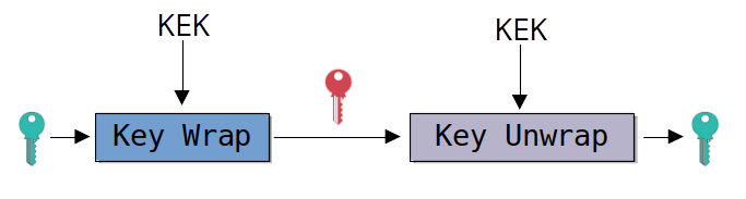
In this article I’ll present you how I attacked an implementation of an AES Key Unwrap (RFC3394) on a Renesas RX65 microcontroller and what I learnt along the way.
The implementation of the correlation algorithm comes from the Chipwhisperer example V4:Tutorial B6 Breaking AES (Manual CPA Attack)
As you might know, when performing SCA, an attacker collects indirect information during the usage of the secret. In my case, the information is electro-magnetic emissions collected outside of the microcontroller with an EM probe.
Because the variance in side-channel emissions correlates to processes within the device, it can leak secrets.
On this target, I can send a command (via the serial communication port) that carries an encryption key to be updated, This new encryption key is protected with the AES key wrap algorithm. In return, I get a response that indicates if the new key was accepted or not.
As the RFC states, “The AES key wrap algorithm is designed to wrap or encrypt key data. The key wrap operates on blocks of 64 bits. Before being wrapped, the key data is parsed into n blocks of 64 bits.”. The key used to do the wrapping will be referred to as the Key-Encryption Key (KEK). That’s the secret that we want to access.
There is no limitation on the number of time that we can send a command to update the key. It means we can try different plaintexts without any limitation. The only limitation is the communication speed, 9600 baud. We can only send 3.5 frames per second. It’s good enough to collect EM traces (40000 traces captures in around 3 hours) but too slow to brute force a lot of key bytes (the brute force is generally performed on a limited number of guesses after the analysis of the traces).
Because I wanted to start in the best conditions, I have a device with:
- a known key,
- a modified firmware that sets a GPIO each time an AES decryption is performed,
Later, in real conditions, the trigger will be based on the end of the serial frame. This will be prone to a lot more jitter.
The AES Key Wrap algorithm operates in blocks of 64 bits (8 bytes). It consists of the following steps:
Split the plaintext key (16 bytes) into 64-bit blocks: P=P1,P2,…,Pn where n (2) is the number of blocks.
Use an initial value (A), often called the
integrity check value (IV), set to a fixed
constant: A=0xA6A6A6A6A6A6A6A6
Concatenate A and the blocks of P to form the initial state: B0=[A,P1,P2,…,Pn]
Perform 6n iterations of AES encryption to securely wrap the key:
for j in range(6): # Outer loop
for i in range(1, n+1): #Inner loop
# - Compute the AES encryption of [A⊕t,Pi]: A,Pi=AESK([A,Pi]) where t=n×j+i.
# - Update A and Pi for each iteration
At the end of the process, A contains the authentication tag, and Pi are the encrypted blocks.
Concatenate A and the encrypted blocks P1,…,Pn to form the wrapped key C: C=[A,P1,P2,…,Pn]
On our target, it’s the opposite operation. The AES Key Unwrap will work on the wrapped key.
At the end of the process, the integrity of the result is checked against the IV.
The AES Key Wrap ensures:
Confidentiality: The key is securely encrypted using AES.
Integrity: The integrity check ensures the wrapped key has not been tampered with.
We want to attack the KEK using SCA. It means that we have to:
send a wrapped key to the device (24 bytes),
compute the first AES plaintext of the Key Unwrap (there are 12 AES operations in total) from the wrapped key,
capture the EM traces during the first AES decrypt
What we send to the device is the input of the key unwrap. What we want is to get the input of the first AES of the key unwrap algorithm. In 4.1 we presented the key wrap in detail. The key unwrap is the same process, but we start from the last indices and also, from the ciphertext. For example.
CIPHER = d6f6a85ee7c27dcd e3cd9ad8af7daabb 4fb8af6f318bd135
P[1]   = e3cd9ad8af7daabb
P[2]   = 4fb8af6f318bd135
A      = d6f6a85ee7c27dcd
During the first key unwrap loop, j = 5 , n = 2 and i = 2 (we start from the final state of the key wrap). The first AES decrypt operation is performed on:
(A ⊕ (n * j + i) || P[2])
= d6f6a85ee7c27dcd ⊕ 0x0c || 4fb8af6f318bd135
= d6f6a85ee7c27dcd ⊕ 0x0c || 4fb8af6f318bd135
= d6f6a85ee7c27dc1 4fb8af6f318bd135
So, the first AES will always be performed on (A ⊕ 12 || P[2])
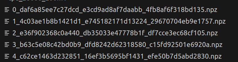
The traces will be saved with the wrapped key in the name and it will start with the index of the trace:
The recovery of the AES input is done during the processing of the traces.
For a complete python implementation of the key unwrap algorithm, see here https://github.com/kurtbrose/aes_keywrap/blob/master/aes_keywrap.py
I’m using a PicoScope 6402C:
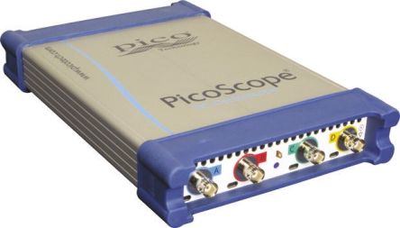
It's a 250MHz scope with 4 channels. The sampling rate is 2.5Gs/s when 2 channels are used. The memory depth is 256M samples total (shared for all channels).
A python API make it easy to control and allow the automatisation of the capture during the transmission of the command frame to the device.
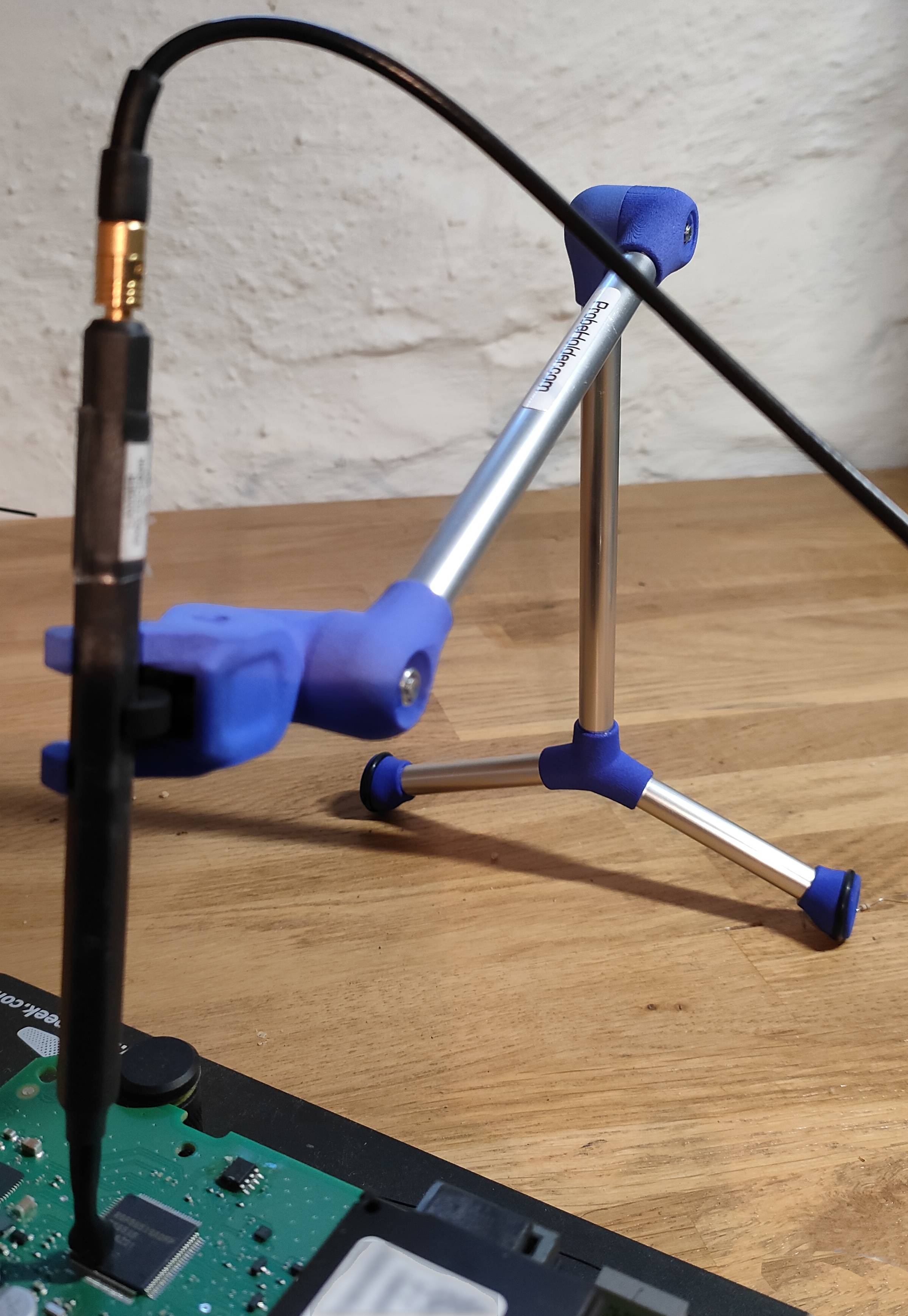
The EM acquisition is done using a LANGER RF U 5-2 probe. It detects the magnetic field:
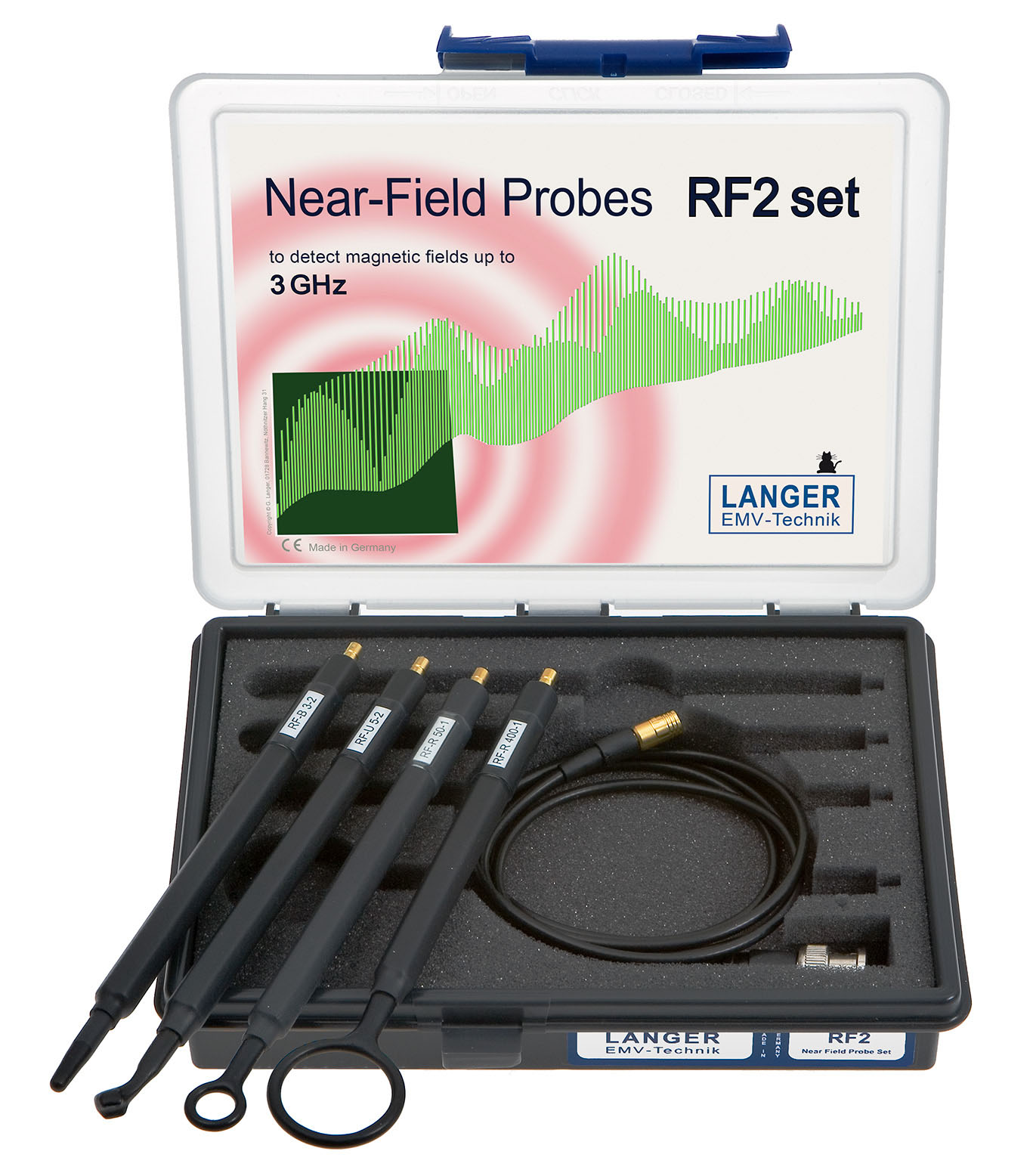
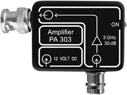
The signal is amplified using a PA203 (30dB):
To find the best spot, I just ran a script that is continuously sending data to the AES key unwrap algorithm and, at the same time, I manually moved the probe from spot to spot. It was easy to visualize on the scope, in real time, where the signal had the highest amplitude:
This is what I get when commands are sent to the device:
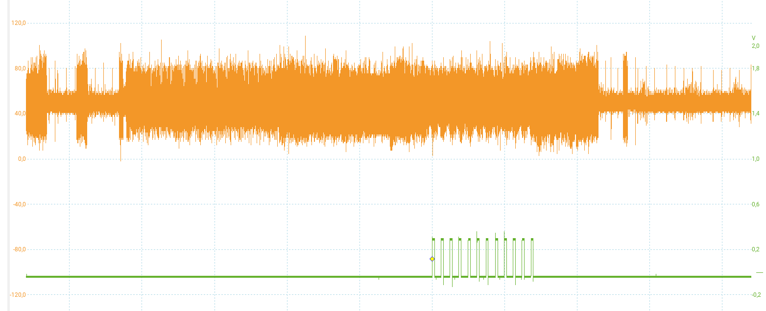
We can see the 12 AES performed by the key unwrap algorithm (in green the trigger for each AES decrypt) and the corresponding EM activity.
What we want now, is to zoom on the first AES and start the capture of traces.
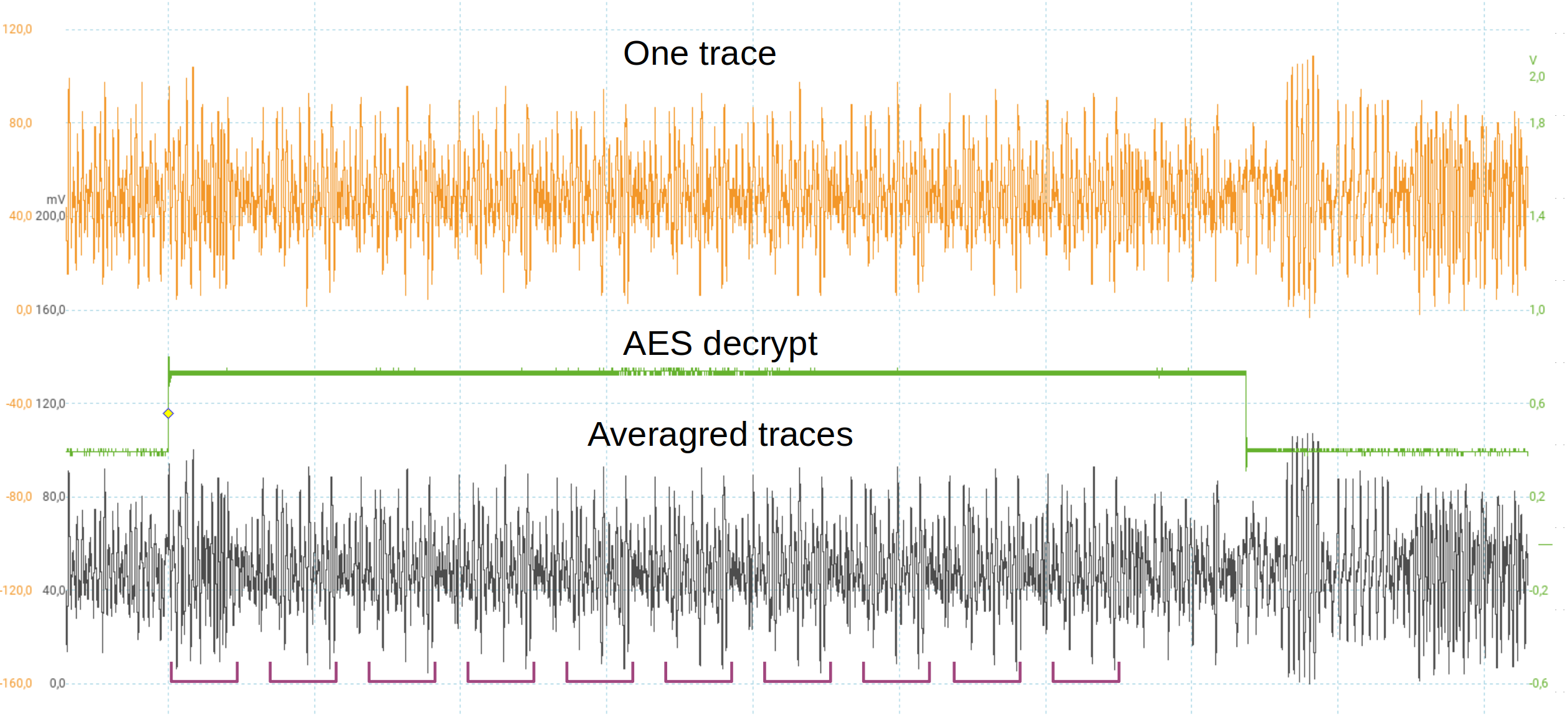
On this capture, to make the AES rounds more visible, the input bandwidth of the scope is limited to 20MHz. On the grey trace, all the realtime captures (orange traces) are averaged.
The 10 AES rounds are clearly visible. We can now start the acquisition of a lot of traces to start the analysis
In the repository here: https://github.com/fjullien/cpa_experiments, you can find the complete test code that is described in this article.
There is also, 100000 traces of 25000 samples captured on my device that you can use to reproduce the results: aes_key_unwrap_100000_traces.tar.xz
As described in chapter 5.1, the name of the traces files (*.npz, NumPy Zip archive) contains the wrapped key that was sent to the device. I wrote a function (load_npz_traces) that:
load trace files,
compute the first AES decrypt cipher from the wrapped key,
can average traces when several captures were done on the same cipher,
returns numpy arrays of cipher and traces.
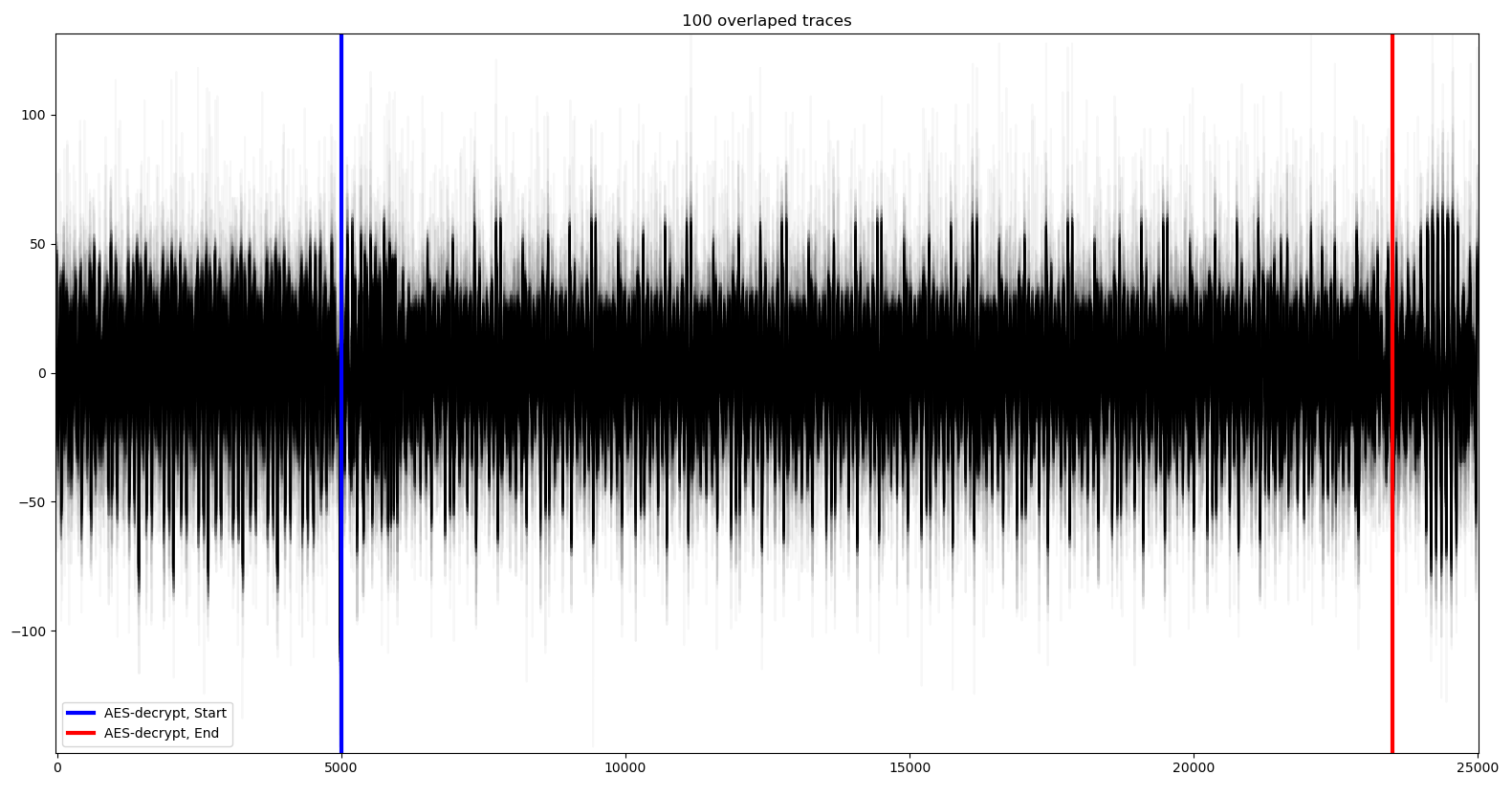
This is what we get once captured and plot with matplotlib (00_plot_traces.py):
python3 00_plot_traces.py --traces ../aes_key_unwrap_100000_traces/ --num 100
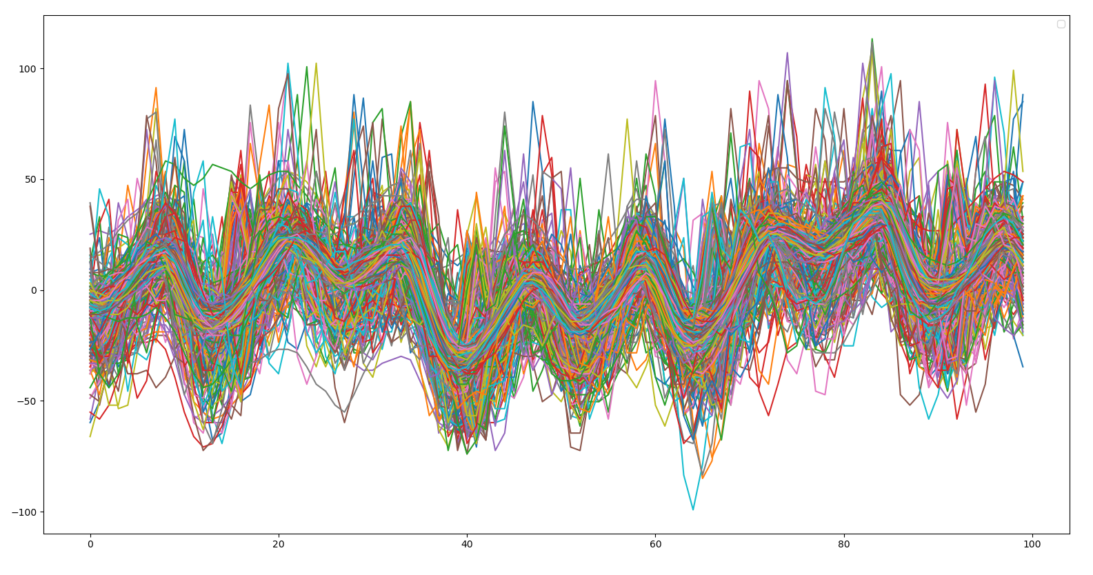
With this view, using alpha blending on traces, we can't really see how noisy the traces are. This is what 3000 traces look like (only showing 100 samples):
In this first example, we will plot 2000 (--num) traces. In each trace, we only consider 7000 (--count) samples starting from 0 (--start).
The alignment will be computed from sample 0 (--sa) to sample 200 (--ea).
The source code is here: 01_frame_alignment.py
python3 01_frame_alignment.py --traces ../aes_key_unwrap_100000_traces --num 2000 --start 0 --count 7000 --sa 0 --ea 200
The first thing that this script does is to plot all the traces over the alignment range [0:200]:
ciphers, traces = cpa_utils.load_npz_traces(num_traces, args.t, sample_start, sample_count)

num_traces, num_samples = traces.shape

for i in range(num_traces):
    plt.plot(traces[i][start_point_for_align:end_point_for_align], alpha=0.03, color="black")
plt.title("Unaligned traces")
plt.show()
As you can see, for whatever reason, the are two groups of traces that are not aligned:
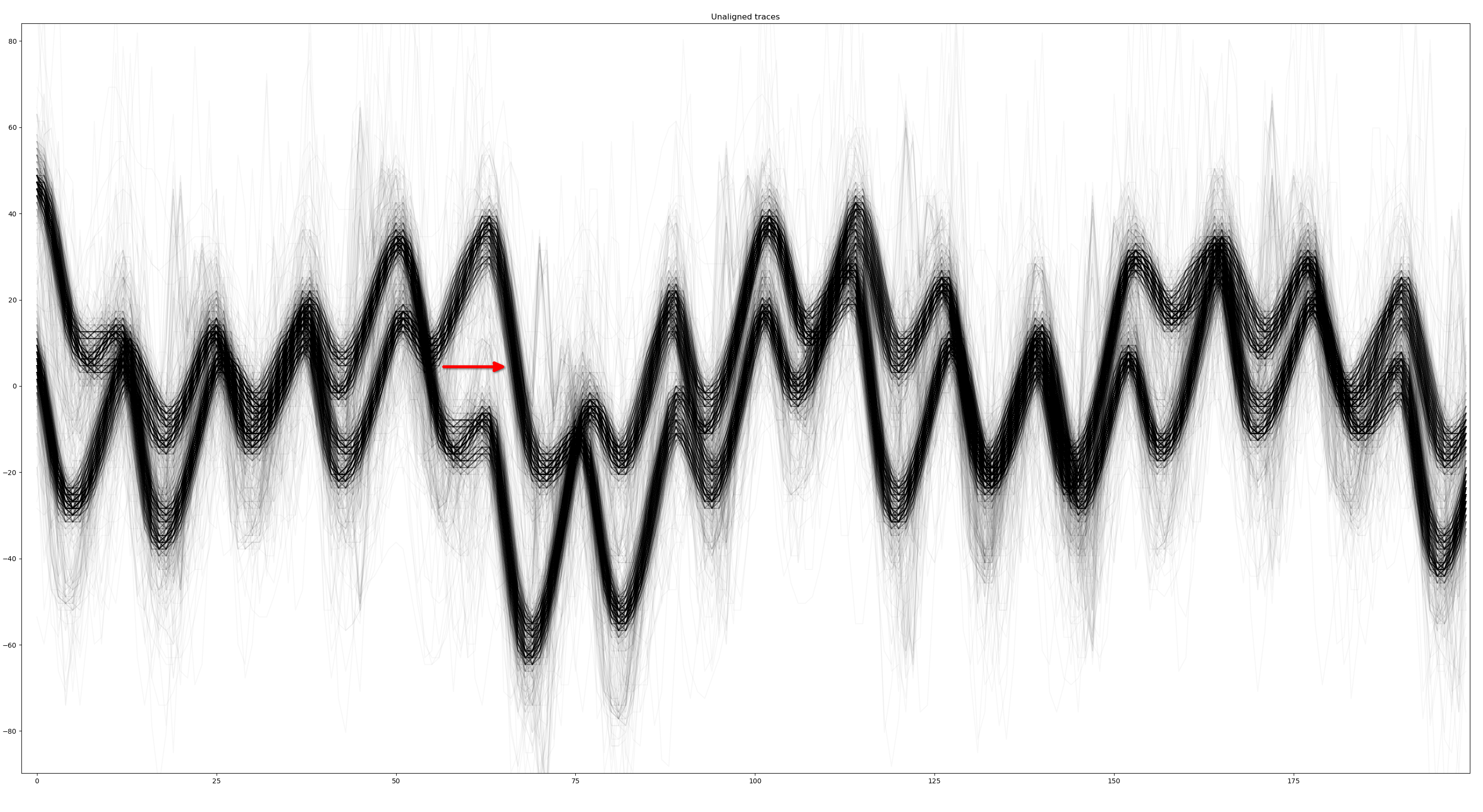
However, we have to be careful here. The traces are not aligned but we're not looking at the position where we would run our analysis. We are focusing on sample [0:2000] but the trigger, where the AES decrypt starts, is at 5000.
It means that traces are unaligned here but the misalignment could be completely different in another part of the trace.
We are first going to illustrate this by aligning the traces based on this range, then we'll look at the result in the area of interest [5000:].
def align_trace(reference, trace, start, end):
    subtrace = trace[start:end]
    correlation = np.correlate(subtrace, reference, mode='full')
    shift = np.argmax(correlation) - (len(subtrace) - 1)
    aligned_trace = np.roll(trace, -shift)
    return aligned_trace

print("Align traces...")

def average_trace(traces, start, end):
    sliced_traces = traces[:, start:end]
    return np.mean(sliced_traces, axis=0)

# We use the first 200 traces to create the reference trace for alignment
averaged_trace  = average_trace(traces[:200], start_point_for_align, end_point_for_align)
# The first trace is arbitrary chosen as reference
reference_trace = traces[0][start_point_for_align:end_point_for_align]

aligned_traces_0   = np.array([align_trace(reference_trace, trace, start_point_for_align, end_point_for_align) for trace in traces])
aligned_traces_avg = np.array([align_trace(averaged_trace, trace, start_point_for_align, end_point_for_align) for trace in traces])
The alignment is performed using cross-correlation (https://en.wikipedia.org/wiki/Cross-correlation) between a reference trace and the trace we want to align.
The trace to be aligned is shifted and the correlation coefficient is computed for each shift. The more the two traces are similar, the higher the coefficient is. So, when we get the higher coefficient, it means that the traces are aligned.
As a reference, we generally use an average of traces. In this example, I also, used an arbitrary trace (the first one, trace[0]) as reference.
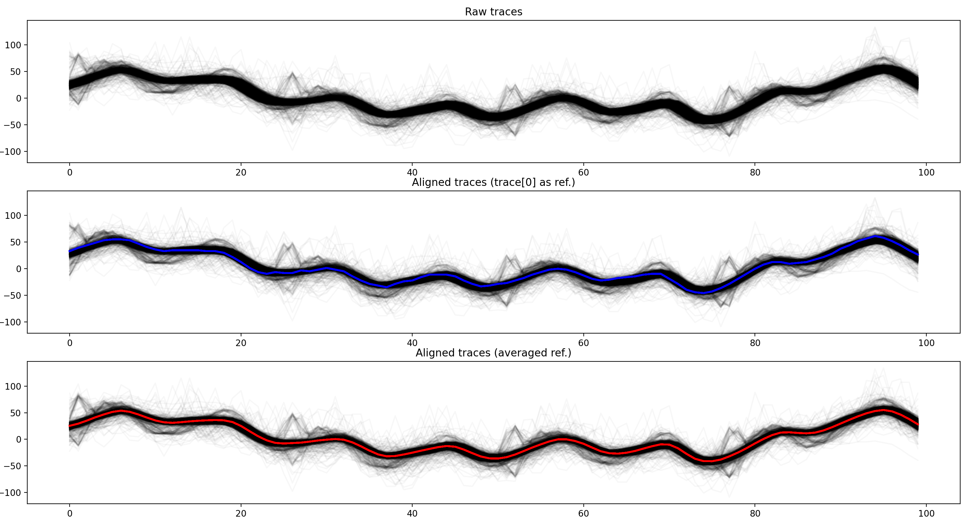
This is the result:
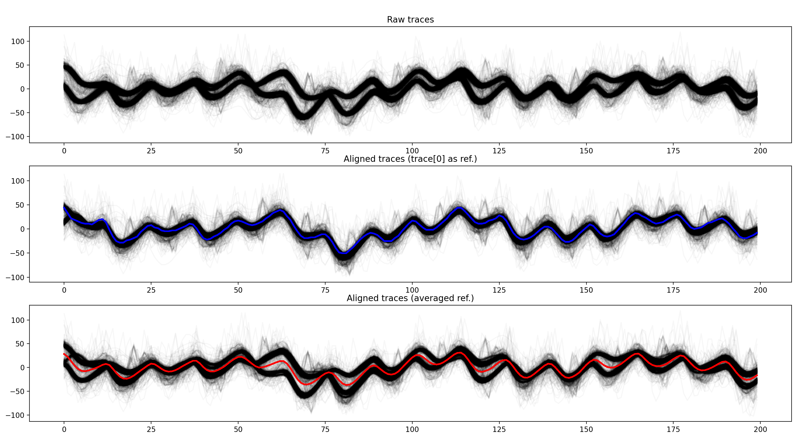
As you can see, because the traces are separated in two distinct groups, the average (red trace) doesn't work very well. The results are better when a single trace is used as a reference.
The alignment works well. In the center plot, all traces are well aligned.
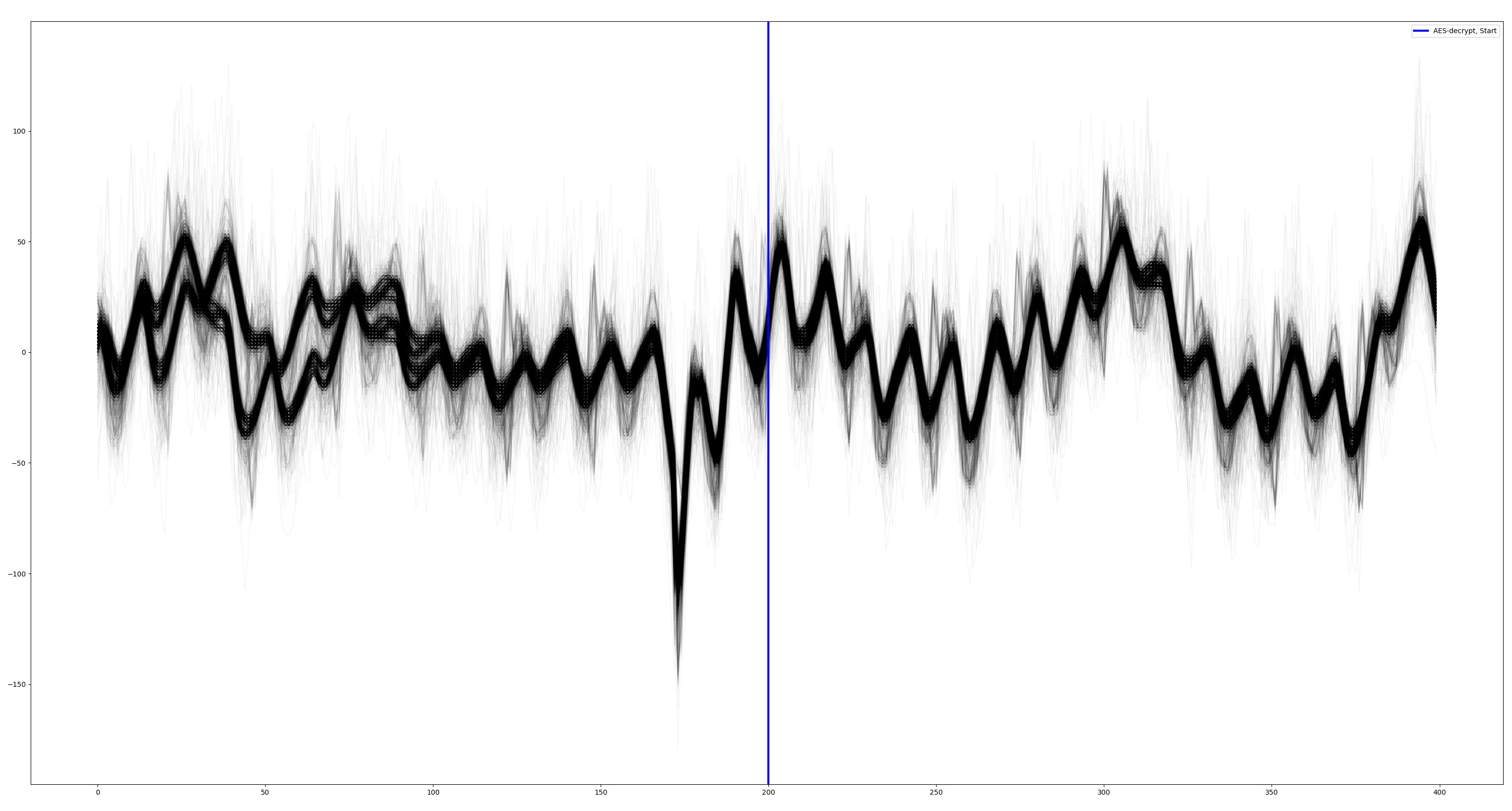
Let's look around the trigger:

The alignment is wrong here! We aligned the traces pre-trigger but, post-trigger it's now unaligned. It shows that we have to be careful when choosing the window for alignment.
This time, let's perform the alignment at [5100:5200], just after the trigger:
python3 01_frame_alignment.py --traces ../aes_key_unwrap_100000_traces --num 2000 --start 0 --count 7000 --sa 5100 --ea 5200
The traces are well aligned even without processing. We use a trigger provided by the firmware itself. It's few instructions just before the AES decrypt So, there is no jitter and the alignment is almost perfect.
When we don't have this, alignment will be required.
Let's look around the trigger:
Now, the traces are well aligned, we can start working on the data.
That's the only thing that we'll do regarding the pre-processing of the traces. We'll see later that filtering, applied to the traces, can improve the results.
I will start with a very short introduction to CPA (Correlation Power Analysis).
When data is manipulated inside the microcontroller, the power consumption is affected by the number of '1' in that data. That's what we call the Hamming weight.
The idea of the CPA is to compare the variation of the power to a model based on the prediction of the hammming weight of a chosen data. If the variation of the two datasets is very small (and there is a linear relation between them), the result of the analysis (correlation coefficient) is a number close to 1 or -1. In that case the model is correct and we have successfully guessed what's happening in the device.
If the two datasets are very different, the coefficient is close to 0, the model is wrong.
As a first experiment, we'll try to see if we can "detect" the input data in the traces. We said that any data on the bus will affect the power.
Before we try to analyze any intermediate state of the AES algorithm, let's just focus on the input of the AES.
Let's say you send 10 plaintexts to the AES decrypt function. We'll focus on the first byte of each ciphertext:
9B E9CF2705BB38ACACEDC23B9F306298
38 92BD1402DF76BDD3A88D66AAAC56F8
78 24CBDDB005CD11D30C220A663BC44B
27 2C97631CC5013AE69C07F808AB5409
C2 972E1EF57C1410BB942B35893280AD
81 2640733B57BB379AAD903831CF5169
4F 74D2A83F41DDB0E448EFC81A473D16
49 342AE3FA99FAE83BAB6D774B3B079C
C4 CF8FFC9B3011FB4DD5C27C963EDB70
86 D26657D9CFF283FF0975B5D4514C8D
Now compute the Hamming weight of each of the first bytes:
[5, 3, 4, 4, 3, 2, 5, 3, 3, 3]
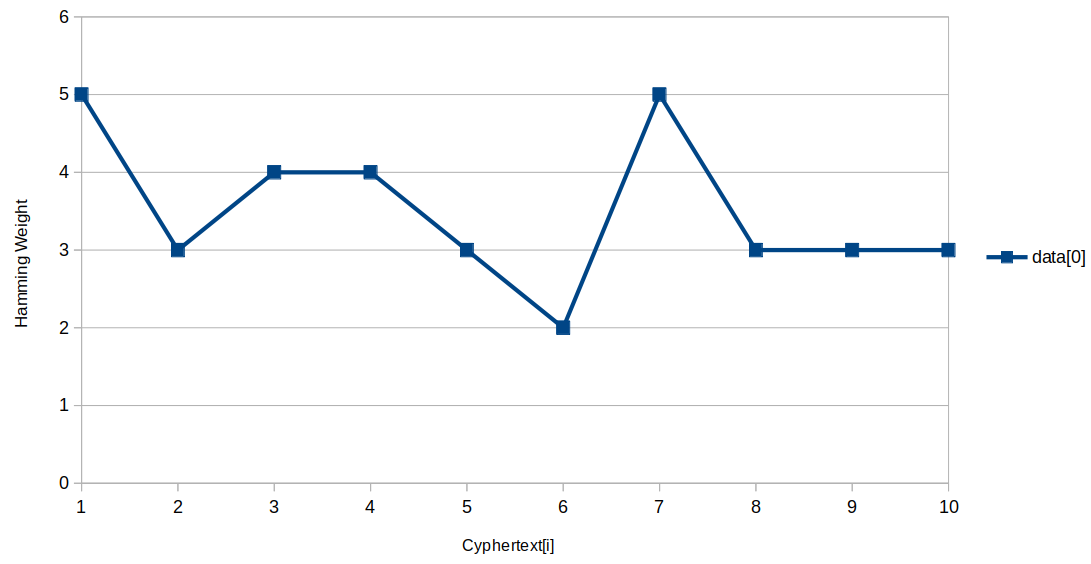
What it means is that there is a point in time, when the first byte of the plaintext is manipulated, where should measure the same variation (or something proportional to this variation) of the power consumption.
So, in this experiment, our model will simply be the Hamming weight of the input value (of one byte because we analyze one key byte at a time).
To compare both data sets (the model and the measurement) we use the Pearson correlation coefficient https://en.wikipedia.org/wiki/Pearson_correlation_coefficient
This formula measures linear correlation between two sets of data:
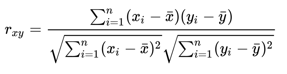
This is how it's implemented in python:
# Compute the hypothesis
for tnum in range(0, num_traces):
    hyp[tnum] = cpa_utils.hw(ciphers[tnum][bnum])

# Mean of hypothesis
meanh = np.mean(hyp, dtype=np.float64)

# Mean of all points in trace
meant = np.mean(aligned_traces, axis=0, dtype=np.float64)

# For each trace, do the following
for tnum in range(0, num_traces):
    hdiff = (hyp[tnum] - meanh)
    tdiff = aligned_traces[tnum,:] - meant
    sumnum = sumnum + (hdiff*tdiff)
    sumden1 = sumden1 + hdiff*hdiff
    sumden2 = sumden2 + tdiff*tdiff

cpaoutput[bnum] = (sumnum / np.sqrt(sumden1*sumden2))
We construct a first dataset made of the samples at a given position of each trace. The second data set is built using the Hamming weight of one of the byte of the input to AES decrypt for the corresponding trace.
Then, we plot the Pearson's coefficient for each sample position. Using 02_cpa_show_leakage.py, we can plot (saved as png files) the CPA results for each bytes of the plaintext:
python3 02_cpa_show_leakage.py --traces ../aes_key_unwrap_100000_traces --num 50000 --start 0 --count 25000 --sa 5500 --ea 5600
Here are the results for bytes 0, 2, and 6 of the input:
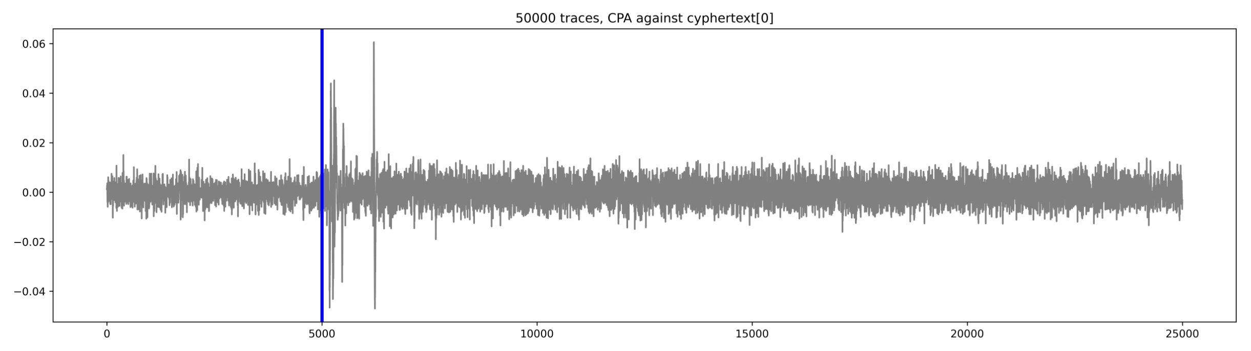
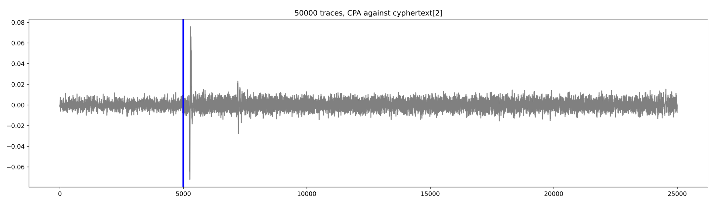
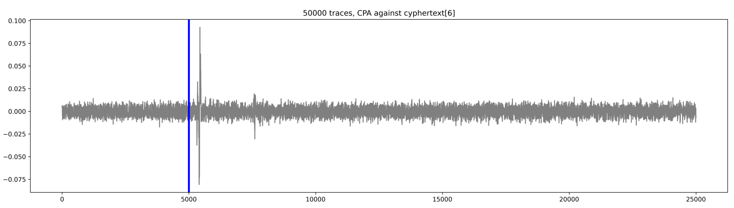
If we plot all results (for all bytes) together, we can clearly see that all the leakage is coming from the first round of the AES decrypt:
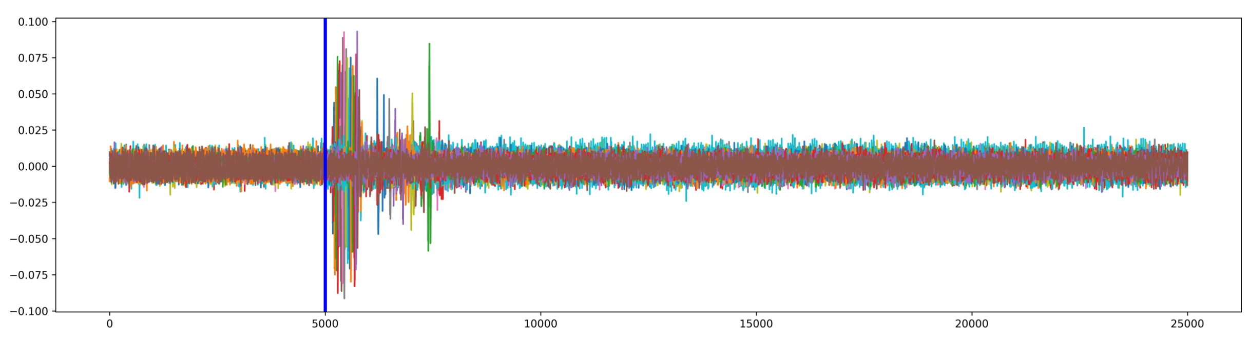
Now we know that the target is leaking information. We demonstrated that the input of the AES decrypt can be leaked. Let's move to the next step.
As you might know, the AES algorithm consists of 10 rounds, where the same sequence of operations is repeated in each round. However, each round requires a unique key derived from the original encryption key, that's the round keys. Round keys are computed during the Key Expansion.
When performing AES decryption, the process essentially reverses the steps of encryption, undoing the transformations applied during the encryption process.
The same key expansion algorithm used during encryption is applied to generate all the round keys. These keys are then used in reverse order during decryption (starting with the last round key).
It means that, because we target the first round of the AES decrypt, if our attack succeed, we'll get the key for the round 10.
I found this tool very useful to get any round key from the base key and vice versa: https://github.com/fanosta/aeskeyschedule.
I know that the KEK of the system that we are studying is:
Known KEK: C2E30C62E54A8F49128F0E005C87467F
Using aeskeyschedule, we can get the key for round 10:
$ aeskeyschedule C2E30C62E54A8F49128F0E005C87467F
0: c2e30c62e54a8f49128f0e005c87467f
1: d4b9de2831f35161237c5f617ffb191e
2: d96dacfae89efd9bcbe2a2fab419bbe4
3: 0987c577e11938ec2afb9a169ee221f2
4: 997a4c7c786374905298ee86cc7acf74
5: 53f0de372b93aaa7790b4421b5718b55
6: d0cd22e2fb5e88458255cc6437244731
7: a66de5785d336d3ddf66a159e842e668
8: 0ae3a0e357d0cdde88b66c8760f48aef
9: ae9d7f33f94db2ed71fbde6a110f5485
10: eebde8b117f05a5c660b84367704d0b3
Once we get key guesses out of the CPA attack, we'll be able to generate the base keys using the same tool.
The decryption process looks like this:
We generally base the model on the output of the inverse S-Box which is an operation inside the decryption round. However, the implementation of the AES decrypt inside our target is a little bit different, it uses look-up tables where the operations of the entire decryption round are all pre-computed.
However, because the input of the table still depends on a single byte of the input, it doesn't change the way that we'll perform the attack. We'll just use the Hamming weight of the table's output (32 bits) to build our model.
Just for fun, I'll briefly show you the software implementation in the actual code.
This is what the decompiled aes_decrypt function looks like:
undefined4 aes_decrypt(byte *output,byte *input,int nb_blocks,byte *key)

{
  int iVar1;
  int iVar2;
  byte round_keys [176];

  iVar1 = key_expansion(round_keys,key);
  if (iVar1 != 0) {
    return 1;
  }
  iVar1 = 0;
  while( true ) {
    if ((nb_blocks & 0xffU) <= iVar1) {
      return 0;
    }
    iVar2 = decryption_rounds(output + (iVar1 * 0x10 & 0xff),input + (iVar1 * 0x10 & 0xff),round_keys,10);
    if (iVar2 != 0) break;
    iVar1 = iVar1 + 1;
  }
  return 1;
}
Round keys are generated as little endian 32 bits words. This is what they look like in memory:
00013678: [0x00] B1 E8 BD EE 5C 5A F0 17 36 84 0B 66 B3 D0 04 77
00013688: [0x10] 36 24 66 0B 81 C9 EC 4F FB F2 16 21 45 0F 4A CF
00013698: [0x20] A7 35 E8 D0 B7 ED 8A 44 7A 3B FA 6E BE FD 5C EE
000136A8: [0x30] 5B 03 E2 EC 10 D8 62 94 CD D6 70 2A C4 C6 A6 80
000136B8: [0x40] 55 33 DB 60 4B DB 80 78 DD 0E 12 BE 09 10 D6 AA
000136C8: [0x50] E2 39 B1 20 1E E8 5B 18 96 D5 92 C6 D4 1E C4 14
000136D8: [0x60] A4 44 1F 2C FC D1 EA 38 88 3D C9 DE 42 CB 56 D2
000136E8: [0x70] A1 60 29 D4 58 95 F5 14 74 EC 23 E6 CA F6 9F 0C
000136F8: [0x80] 65 7C 2D D6 F9 F5 DC C0 2C 79 D6 F2 BE 1A BC EA
00013708: [0x90] 96 2E 2A 09 9C 89 F1 16 D5 8C 0A 32 92 63 6A 18
00013718: [0xA0] 62 0C E3 C2 49 8F 4A E5 00 0E 8F 12 7F 46 87 5C
Then, during the decryption rounds we first do the AddRoundKey (input xor last round key):
Input of AES decrypt (ciphertext): 24 CA 12 AF 0C 9A 03 6F BF 38 55 4A 2A D3 4B 94
AES Key                          : C2 E3 0C 62 E5 4A 8F 49 12 8F 0E 00 5C 87 46 7F

[R14] (Last round key)           : B1 E8 BD EE 5C 5A F0 17 36 84 0B 66 B3 D0 04 77

r01 : 24ca12af
r03 : bf38554a
r04 : 0c9a036f
r06 : 2ad34b94

fff26dfa 06 a0 0d e1   XOR    [R14].L, R1
fff26dfe 62 4e         ADD    # 0x4, R14
fff26e00 06 a0 0d e4   XOR    [R14].L, R4
fff26e04 62 4e         ADD    # 0x4, R14
fff26e06 06 a0 0d e3   XOR    [R14].L, R3
fff26e0a 62 4e         ADD    # 0x4, R14
fff26e0c 06 a0 0d e6   XOR    [R14].L, R6
fff26e10 62 4e         ADD    # 0x4, R14

Output of AddRoundKey:

r01 : ca77fa1e
r03 : d933d17c
r04 : 1b6a5933
r06 : 5dd79b27
The output of AddRoundKey will normally go to InverseShiftRows, InvSubBytes, InvMixColumns. However the target uses Golang's implementation which uses precomputed values (T-Tables) to optimizes the AES algorithm.
You can find a very good explanation here: https://blog.tclaverie.eu/posts/understanding-golangs-aes-implementation-t-tables/
In this article, there is a decryption code that uses T-Tables:
func decrypt(src []uint32, xk []byte, nr int) []byte {
    ...
    // Add the last round key to the state
    s0 ^= xk[nr*4]
    s1 ^= xk[nr*4+1]
    s2 ^= xk[nr*4+2]
    s3 ^= xk[nr*4+3]

    for i:= nr-1; i > 0; i-- {
        // This performs InvShiftRows + InvSubBytes + AddRoundKey + InvMixColumns
        tmp0 = td0[s0>>24] ^ td1[s3>>16&0xff] ^ td2[s2>>8&0xff] ^ td3[s1&0xff] ^ xk[4*i]
        ...
With r01, r03, r04 and r06 being respectively s0, s2, s1 and s3, we can see that the disasembly matches exactly the function here above:
              LAB_fff26e17                                        fff26f6d(j)
  fff26e17 fb 22 cc 19 f4 ff      MOV.L        XREF[1]:   #AES_Td0, R2
  fff26e1d fd 98 17               SHLR                    # 0x18, R1, R7            // [0xCA] (s0 >> 24)
  fff26e20 fe 67 27               MOV.L                   [R7, R2]=>AES_Td0, R7

  fff26e23 fb 22 cc 19 f4 ff      MOV.L                   #AES_Td0, R2
  fff26e29 fd 90 68               SHLR                    # 0x10, R6, R8
  fff26e2c 76 28 ff 00            AND                     #0xff, R8                 // [0xD7] (s3 >> 16)
  fff26e30 fe 68 22               MOV.L                   [R8, R2]=>AES_Td0, R2

  fff26e33 fd 6c 82               ROTR                    # 0x8, R2
  fff26e36 fc 37 27               XOR                     R2, R7

  fff26e39 fb 22 cc 19 f4 ff      MOV.L                   #AES_Td0, R2
  fff26e3f 5f 38                  MOVU.W                  R3, R8
  fff26e41 5f 88                  MOVU.W                  R8, R8
  fff26e43 68 88                  SHLR                    # 0x8, R8                 // [0xD1] (s2 >> 8)
  fff26e45 fe 68 22               MOV.L                   [R8, R2]=>AES_Td0, R2

  fff26e48 fd 6f 02               ROTL                    # 0x10, R2
  fff26e4b fc 37 27               XOR                     R2, R7

  fff26e4e fb 22 cc 19 f4 ff      MOV.L                   #AES_Td0, R2
  fff26e54 ef 48                  MOV.L                   R4, R8
  fff26e56 76 28 ff 00            AND                     #0xff, R8                 // [0x33] (s1 >> 0)
  fff26e5a fe 68 22               MOV.L                   [R8, R2]=>AES_Td0, R2

  fff26e5d fd 6e 82               ROTL                    # 0x8, R2
  fff26e60 fc 37 27               XOR                     R2, R7
  fff26e63 06 a0 0d e7            XOR                     [R14].L, R7               // [R14] is the round key
  fff26e67 62 4e                  ADD                     # 0x4, R14
  ....
Performing the attack is almost exactly what we've done in chapter 7, when we were looking for leakage.
This time, we won't use the input bytes to model the leakage but we'll use the output of the T-Table. We saw that each byte of the ciphertext is first XORed with the round key then used as an input of the T-Table.
It means that we can use the output of the T-Table to find the best guess of each bytes of the key.
We'll use this script: 03_cpa_attack.py
The T-Table is present in cpa_utils.py and a precomputed table with the Hamming weight of the output for any input byte can be obtained with hw_t_table_decrypt():
t_table_decrypt = [
    0x50, 0xa7, 0xf4, 0x51, 0x53, 0x65, 0x41, 0x7e, 0xc3, 0xa4, 0x17, 0x1a, 0x96, 0x5e, 0x27, 0x3a,
    0xcb, 0x6b, 0xab, 0x3b, 0xf1, 0x45, 0x9d, 0x1f, 0xab, 0x58, 0xfa, 0xac, 0x93, 0x03, 0xe3, 0x4b,
    ...
    0x71, 0x01, 0xa8, 0x39, 0xde, 0xb3, 0x0c, 0x08, 0x9c, 0xe4, 0xb4, 0xd8, 0x90, 0xc1, 0x56, 0x64,
    0x61, 0x84, 0xcb, 0x7b, 0x70, 0xb6, 0x32, 0xd5, 0x74, 0x5c, 0x6c, 0x48, 0x42, 0x57, 0xb8, 0xd0
]

# Return a precomputed table with the Hamming weight of the T-Table output for each possible input values)
def hw_t_table_decrypt():
    return [hw(t_table_decrypt[i*4]) + hw(t_table_decrypt[(i*4)+1]) + hw(t_table_decrypt[(i*4)+2]) + hw(t_table_decrypt[(i*4)+3]) for i in range(256)]
This is how we build the leakage model. For an input byte, we xor it with the round key then we compute the HW on the output of the T-Table:
#-----------------------------------------------------------------------
# This is our model. We return the Hamming weight of the result of:
# - cipher xor keyguess (which is AddRoundKey)
# - output of the table with the input equal to the above result
#-----------------------------------------------------------------------
def intermediate(ciphertext_byte, keyguess):
    return t_table_hw_dec[ciphertext_byte ^ keyguess]
Now we can start the attack. This is what the script does:
# Load traces
...

# Align traces
...

#-----------------------------------------------------------------------
# This is our model. We return the Hamming weight of the result of:
# - cipher xor keyguess (which is AddRoundKey)
# - output of the table with the input equal to the above result
#-----------------------------------------------------------------------
def leakage_model(ciphertext_byte, keyguess):
    return t_table_hw_dec[ciphertext_byte ^ keyguess]

...

# Number of key bytes we want to attack
BNUM = 16

# We attack each byte individualy
for bnum in range(0, BNUM):

    ...

    with Bar(f'Attacking key byte {bnum}', max=256) as bar:

        # For each guess of a key byte, we compute the coefficients
        for kguess in range(0, 256):

            # Get the trace and the max. coeff. value
            cpaoutput[kguess], maxcpa[kguess] = cpa_utils.compute_coeff(bnum, kguess, plaintexts, leakage_model, aligned_traces)

        # Sort the guesses by their coefficient (only the first 32)
        ...

        # Print the six best key guesses and their coefficient. Highlight the known key byte if present
        ...

        # Print the 32 best key guesses
        ...

        # Plot the correlation coefficient for each sample for the 6 best guesses
        ...

# Print complete guessed key
...
python3 03_cpa_attack.py --traces aes_key_unwrap_100000_traces/ --num 50000 --start 5500 --count 2500 --sa 100 --ea 200
Let's have a look at the results. This is what we get for byte 0:
We get a pretty good correlation on the first key byte. However, for some of the bytes, the correlation is strong but the result is not correct:
Even with more traces, the ranking of the correct key byte doesn't change.
We finally get 11 out of 16 bytes of the key:

Of course, at this point, we could evaluate how strong is the confidence for each byte of the key and decide how much of the top guesses we need to be sure to pick the right key byte.
Once we have a list of each candidate for each key byte, we can start a brute force attack to recover the key.
Even if we blindly choose the four top guesses for each key byte, we get "only" 4^16 possible keys which is not a lot.
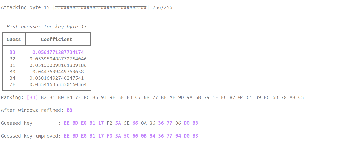
During my tests, I realized that the first peak of correlation always gave the correct key byte. For example, for byte 10, the highest coefficient gives a key value of 0x86. However, the correct key byte is 0x84.
If we look closely at the traces, this is what we see:
I improved the attack script to detect peaks and choose the best candidate inside a window around the first peak.
On the plot hereabove, you can see the noise level that is evaluated on the first 500 samples. Then, each red cross identify a peak (it uses find_peaks of scipy.signal).
The evaluation window is 20 samples wide and centered around the first peak.
Once we run the script with the new improvement (04_cpa_attack_improved.py) we finally get the correct key:
python3 04_cpa_attack_improved.py --traces aes_key_unwrap_100000_traces/ --num 50000 --start 5500 --count 2500 --sa 100 --ea 200
The peak detection is far from perfect. It's just a toy. The most efficient way would be to manually extract the location of the first peak for each key byte and perform a cpa on these locations only. That would also, speed-up the search as the number of samples would be reduced a lot.
The last point I want to cover now is the evolution of the correlation coefficient with the number of traces.
We'll plot convergence traces to determine how many traces are needed to guess the correct key.
The script 05_convergence_plot.py is used to plot the convergence graph.
It uses compute_coeff_with_convergence() that returns a list of coefficients for each trace count from 1 to the total number of traces. Then we can plot it and see how the coefficient changes with the number of traces analyzed.
With this, we can visualize how many traces are needed to get to a clear identification of the correct guess.
This is for example the byte 10 analyzed up to 50000 traces (I limited the traces to 20 samples):
python3 05_convergence_plot.py --traces aes_key_unwrap_100000_traces/ --num 50000 --start 6350 --count 20 --sa 0 --ea 20
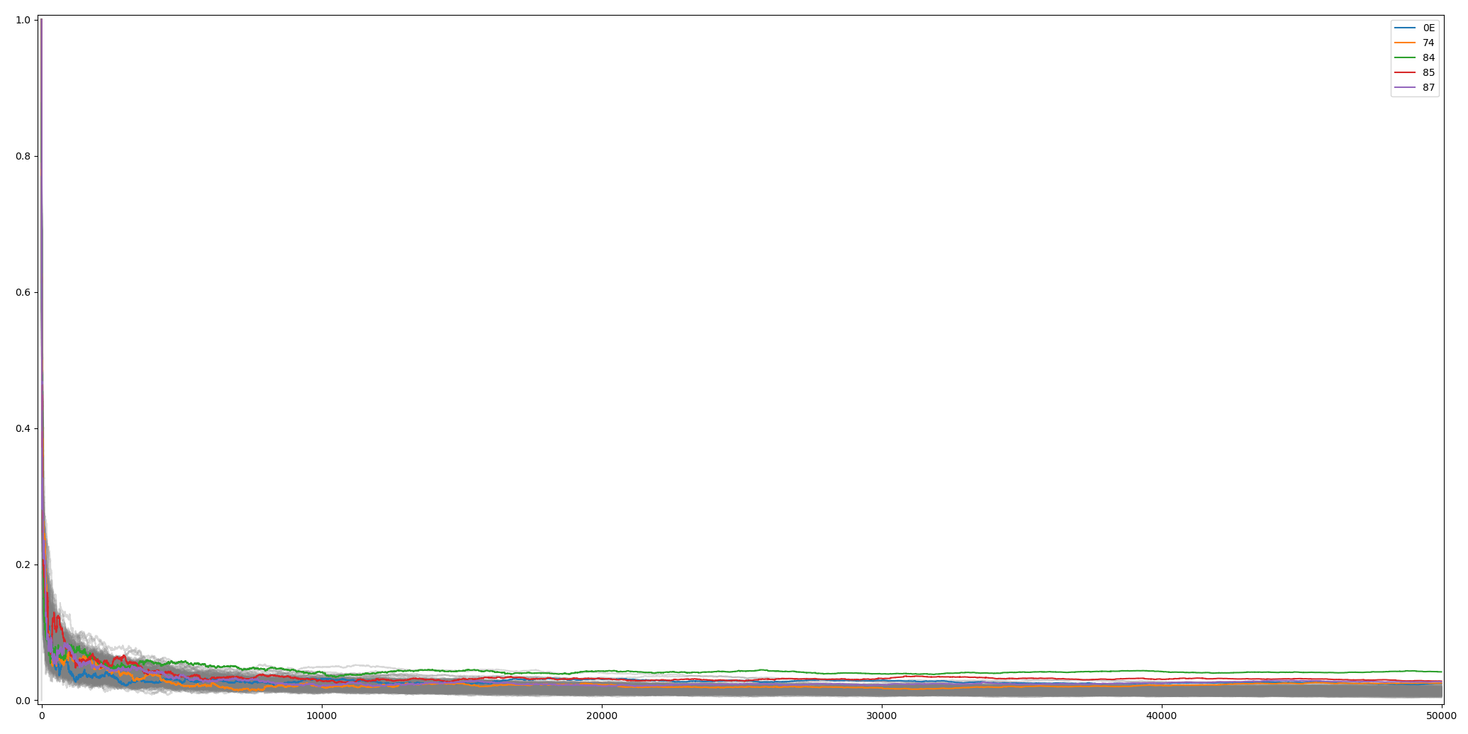
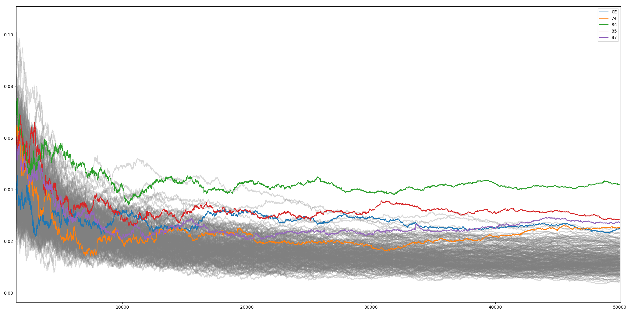
The green traces represent byte 0x84 (the good guess). From sample 25000, the trace is really separated from the others. That's the minimum number of traces required to get to the result.
In order to improve the correlation, a filter can be applied to the traces. We can for example use a Savitzky-Golay filter https://en.wikipedia.org/wiki/Savitzky-Golay_filter to reduce the noise.
In the example 06_convergence_plot_with_filter.py I choose to do the CPA on byte 10 of the key using only the 4 best guesses that we got from the previous experiments.
We then plot the convergence plot for different filters applied to the traces:
    print("Filter traces...")

    filtered_traces = np.empty_like(traces)
    window_length = 17 # Choose a suitable window length (must be odd)
    polyorder = 4  # Choose the order of the polynomial fit
    for i in range(num_traces):
        filtered_traces[i] = savgol_filter(aligned_traces[i], window_length, polyorder)

    filtered_traces_11 = np.empty_like(traces)
    window_length = 11 # Choose a suitable window length (must be odd)
    polyorder = 4  # Choose the order of the polynomial fit
    for i in range(num_traces):
        filtered_traces_11[i] = savgol_filter(aligned_traces[i], window_length, polyorder)

    ...

    cpa_tests = {
        "Non filtered"             : (aligned_traces,     [0]*256, [0]*256, [0]*256, "blue"),
        "Filtered, WL=17, Order=4" : (filtered_traces,    [0]*256, [0]*256, [0]*256, "green"),
        "Filtered, WL=11, Order=4" : (filtered_traces_11, [0]*256, [0]*256, [0]*256, "red"),
    }

    ...

    key_guess_list = [0x84, 0xcb, 0xd6, 0x0e]

    # Perform the CPA and plot the result for each group of traces
    for traces_type in cpa_tests:
        traces, cpaoutput, maxcpa, cpa_evol, color = cpa_tests[traces_type]
        with Bar(f"Attacking key byte {bnum}", max=len(key_guess_list)) as bar:
            for kguess in key_guess_list:
                cpaoutput[kguess], maxcpa[kguess], cpa_evol[kguess] = cpa_utils.compute_coeff_with_convergence(bnum, kguess, plaintexts, leakage_model, traces)
                bar.next()
    ...
python3 06_convergence_plot_with_filter.py --traces aes_key_unwrap_100000_traces/ --num 50000 --start 6300 --count 70 --sa 0 --ea 20
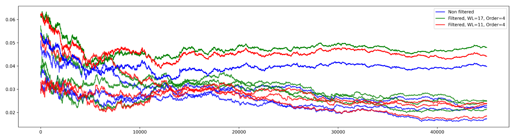
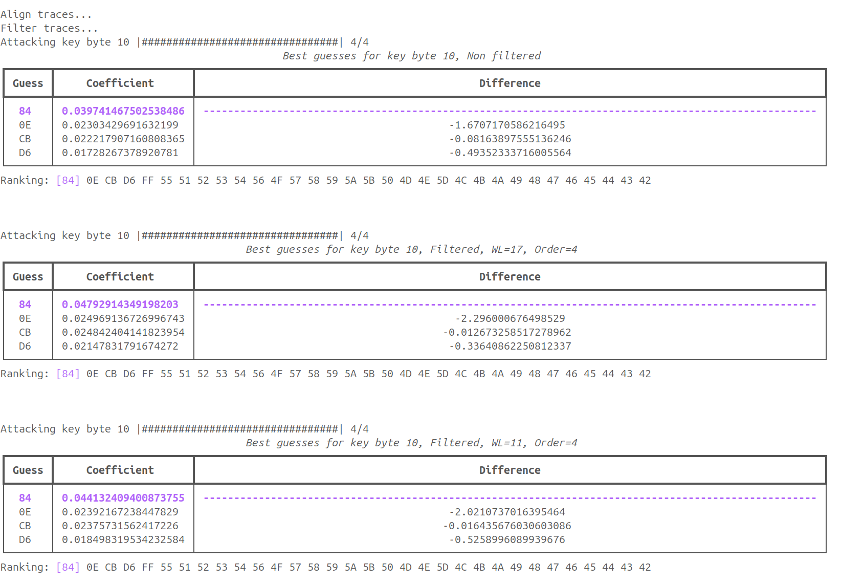
We observe a slight improvement when the traces are filtered. The distance between the good guess and the others guesses is more important with the filter (green trace, window length = 17, polyome order = 4).
It's also visible in the table where I added a column that shows the difference (x100) between two successive coefficients.
It might be interesting to redo the experiment with the script 04_cpa_attack_improved.py but this time with a filter applied on the traces.
We could also, reduce the number of traces to see where the effect of the filter starts to be visible on the results.
I won't do it now :)
I've shown that we can recover the KEK when traces are captured in the best conditions (with a GPIO that indicates where the AES starts).
Next, I'll try to do the same thing using a complete black box approach where I don't have access to the firmware (and the KEK) and I can only synchronize the traces with the frame that is sent on the serial port. The synchronization of the trigger point will be a lot harder and the alignment of the traces will be then more challenging.
Stay tuned!
Franck Jullien - 2025
Follow me on X and Bluesky! @fjullien06, fjullien.bsky.social